COMP9417 - Machine Learning

Tutorial: Regression II

Question 1. Maximum Likelihood Estimation (MLE)

In this question we will first review and then work through a few examples of parameter estimation using the MLE technique. The following introduction can be skipped if you are comfortable with the MLE concept already.

The setting is as follows: we sample n observations (data), which we denote by X₁,X₂,...,X_n, and we assume that the data is independently drawn from some probability distribution P. The shorthand for this is:

i.i.d.

X₁,...,X_n ∼ P,

where i.i.d. stands for independent and identically distributed. In practice, we never have access to P, we are just able to observe samples from P (namely X₁,...,X_n), which we will use to learn something about P. In the simplest case, we assume that P belongs to a parametric family. For example, if we assume that P belongs to the family of normal distributions, then we are assuming that P has a probability density function (pdf) of the form

,

where we will usually refer to µ as the mean, and σ² as the variance, and we combine all unkown parameters into a single parameter vector θ that lives in some parameter space Θ. In this particular example, Θ = R × [0,∞). Under this assumption, if we knew θ, then we would know P, and so the learning problem reduces to learning the best possible parameter θ^∗, hence the name parametric.

Continuing with this example, we need a way of quantifying how good a particular choice of θ is. To do this, we first recall the fact that for independent sets A,B,C, it holds that P(A and B and C) = P(A)P(B)P(C). Therefore, we have:

Prob of observing X₁,...,X_n = Prob of observing X₁ × ··· × Prob of observing X_n

=:

We call L(θ) the likelihood, and it is a function of the parameter vector θ. We interpret this quantity as the probability of observing the data when using a particular choice of parameter. Obviously, we want to

1

choose the parameter θ that gives us the highest possible likelihood, i.e. we wish to find the maximum

likelihood estimator

θ^ˆ_MLE := argmaxL(θ).

θ∈Θ

Since this is just an optimization problem, we can rely on what we know about calculus to solve for the MLE estimator.

i.i.d.

• Assume that X₁,...,X_n ∼ N(µ,1), that is, we already know that the underlying distribution is Normal with a population variance of 1, but the population mean is unkown. Compute µˆ_MLE.

Hint: it is often much easier to work with the log-likelihood, i.e. to solve the optimisation:

θ^ˆ_MLE := argmaxlogL(θ),

θ∈Θ

which gives exactly the same answer as solving the original problem (why?). i.i.d.

• Assume that X₁,...,X_n ∼ Bernoulli(p), compute pˆ_MLE. Recall that the Bernoulli distribution is discrete and has probability mass function:

P(X = k) = p^k(1 − p)^1−k, k = 0,1 p ∈ [0,1].

i.i.d. ²). Compute.

• optional: Assume that X₁,...,X_n ∼ N(µ,σ

Question 2. Bias and Variance of an Estimator

In the previous question, we discussed the MLE as a method of estimating a parameter. But there are an infinite number of ways to estimate a parameter. For example, one could choose to use the sample median instead of the MLE. It is useful to have a framework in which we can compare estimators in a systematic fashion, which brings us to two central concepts in machine learning: bias and variance. Assume that the true parameter is θ, and we have an estimate θ^ˆ. Note that an estimator is just a function of the observed (random) data (i.e. we can always write θ^ˆ = θ^ˆ(X)) and so is itself a random variable! We can therefore define:

bias(θˆ) = E(θˆ) − θ,

var(θˆ) = E(θˆ− E(θˆ))².

The lab this week explores these concepts as well, and you are encouraged to do the lab exercise as you complete this question to get a full picture. A short summary of the lab in words:

bias: tells us how far the expected value of our estimator is from the truth. Recall that an estimator is a function of the data sample we observe. The expectation of an estimator can be thought of in the following manner: imagine instad of having a single data sample, we have an infinite number of data samples. We compute the same estimator on each sample, and then take an average. This is the expected value of the estimator.

• varaiance: how variable our estimator is. Again, if we have an infinite number of data samples, we would be able to compute the estimator an infinite number of times, and check the variation in the estimator across all samples.

A good estimator should have low bias and low variance.

i.i.d.

Find the bias and variance of µˆ_MLE where X₁,X₂,...,X_n ∼ N(µ,1).

i.i.d.

Find the bias and variance of pˆ_MLE where X₁,X₂,...,X_n ∼ Bernoulli(p).

• The mean squared error (MSE) is a metric that is widely used in statistics and machine learning.

For an estimator θ^ˆ of the true parameter θ, we define its MSE by:

MSE(θˆ) := E(θˆ− θ)².

Show that the MSE obeys a bias-variance decomposition, i.e. we can write

MSE(θ^ˆ) := bias(θ^ˆ)² + var(θ^ˆ).

Question 3. Probabalistic View of Least-Squares regression

In the tutorial last week, we viewed the least-squares problem purely from an optimisation point of view. We specified the model we wanted to fit, namely:

yˆ = w^Tx

as well as a loss function (MSE), and simply found the weight vector w that minimized the loss. We proved that when using MSE, the best possible weight vector was given by

wˆ = (X^TX)⁻¹X^Ty.

In this question, we will explore a different point of view, which we can call the statistical view. At the heart of the statistical view is the data generatinc process (DGP), which assumes that there is some true underlying function that generates the data, which we call f, but we only have access to noisy observations of f. That is, we observe

is some random noise.

For example, assume your y’s represent the daily temperature in Kensington. Any thermometer - even the most expensive - is prone to measurement error, and so what we actually observe is the true temperature (f(x)) plus some random noise . Most commonly, we will assume that the noise is normally distributed with zero mean, and variance σ². Now, consider the (strong) assumption that f(x) is linear, which means that there is some true β^∗ such that f(x) = x^Tβ^∗. Therefore, we have that

,

and therefore,

y|x ∼ N(x^Tβ^∗,σ²).

What this says is that our response (conditional on knowing the feature value x) follows a normal distribution with mean x^Tβ^∗ and variance σ². We can therefore think of our data as a random sample of observations coming from this distribution, which in turn allows us to estimate unknown parameters via maximum likelihood, just as we did in the previous questions.

(a) You are given a dataset D = {(x₁,y₁),...,(x_n,y_n)} and you make the assumption that y_i|x_i = for some unknown β^∗ and, where all the _i’s are independent of each other. Write down the log-likelihood for this problem as well as the maximum likelihood estimation objective and solve for the MLE estimator β^ˆ_MLE.

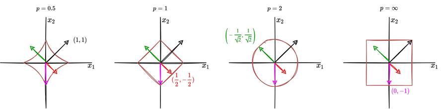
Question 4. Geometric Interpretations

In this question we will explore some geometric intuition for the least squares (LS), ridge and LASSO regression models.

• Consider the following diagram which represents the contour plot of the unit ball under various pnorms (see lab0 if you are unfamiliar with contour plots). Explain what is going on, and comment√ √

on the four vectors ((1,1),(1/2,−1/2),(−1/ 2,1/ 2),(0,−1)) that are represented in the plots. Further, what is the difference between the first plot (p = 0.5) and the others?

• We previously saw that the ridge regression objective is defined by:

βˆridge = argmin .

Another (equivalent) way of defining the ridge objective is through a constrained optimisation:

β^ˆ_ridge = argmin subject to kβk₂ ≤ k.

What this says is that we want to find β that minimizes the squared loss but the solution must also belong to the 2-norm ball of radius k. Note that in general, k and λ are not the same. The constrained optimisation statement gives us a nice geometric interpretation of the ridge solution which we will now explore. Before doing so, we also note that the LASSO has an unconstrained version:

βˆLASSO = argmin .

and also a constrained version

β^ˆ_LASSO = argmin subject to kβk₁ ≤ k,

where λ,k for the Ridge and for the LASSO are different in general. These objectives are almost identical, they only differ by the choice of norm used for the penalty/constraint term. This actually leads to large and very important differences in practice. Now, with this in mind, interpret the following plots:

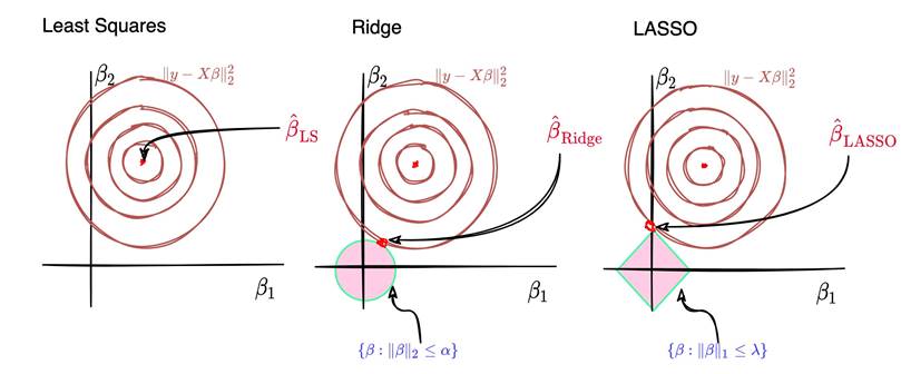
Discuss the differences in the Ridge and LASSO solutions explicitly.

(c) The LASSO is said to induce sparsity. What does this mean? Why might it be desirable to have a sparse solution?